Precise embedded profiling with VisualGDB
This tutorial shows how to do an in-depth performance analysis of your embedded code using the VisualGDB instrumenting profiler. Unlike the sampling profiler that only takes measurements from time to time, the instrumenting profiler precisely measures the time taken by each function call. This produces more overhead, but allows collecting very high-precision profiling data. The profiler currently supports only the ARM Cortex devices with the THUMB instruction set.
Before you begin, install VisualGDB 5.1 or later.
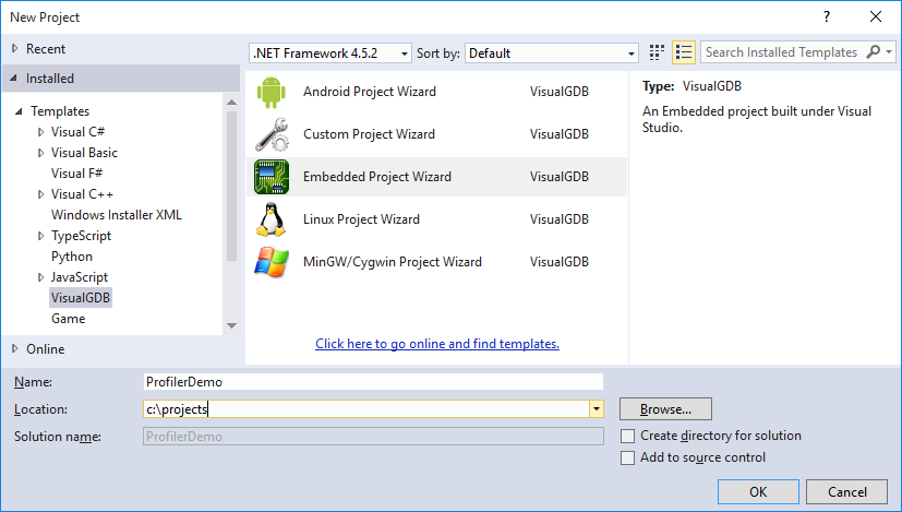
- Start Visual Studio and open the VisualGDB Embedded Project Wizard:
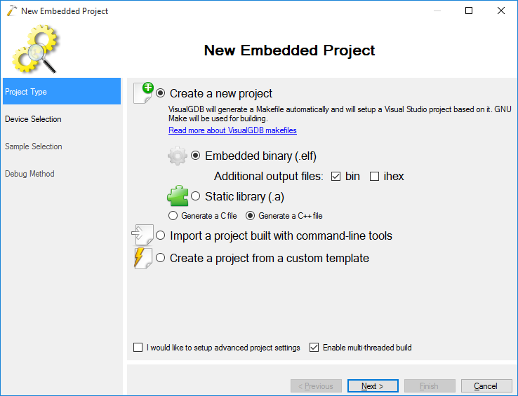
- Select “Embedded binary” on the first page:
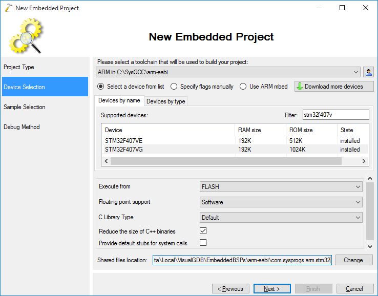
- On the next page select the ARM toolchain and choose your device. We will demonstrate the profiling on the STM32F4-Discovery board, however any other ARM device that supports debug instruction counter will do as well:
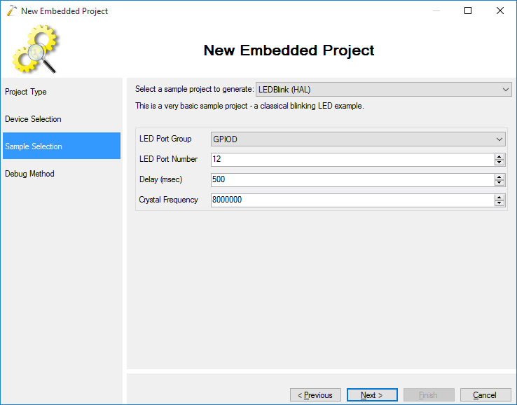
- Proceed with the default “LEDBlink” sample:
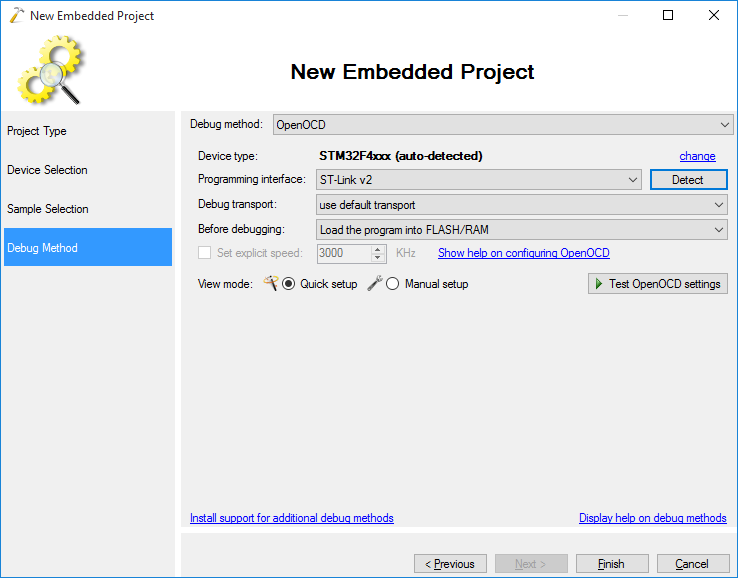
- Finally select the debug method that works with your board. For the STM32 devices we recommend using OpenOCD:
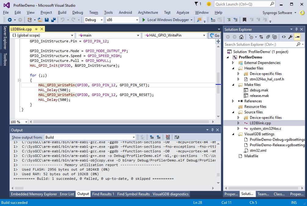
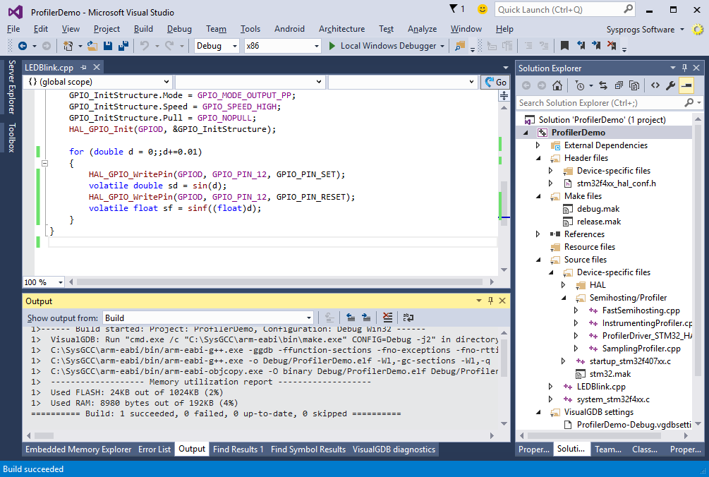
- Press “Finish” to create your project. Build it by pressing Ctrl-Shift-B:
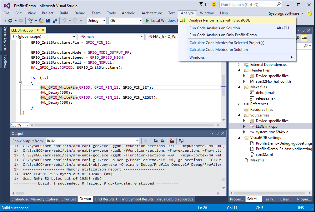
- Run the “Analyze Performance with VisualGDB” command from the “Analyze” menu :
- VisualGDB will suggest adding a reference to the profiler framework. Select “Yes”:
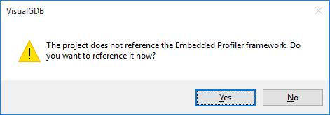
- Initialize the profiling framework from your code by including <SysprogsProfiler.h> from your main source file and calling InitializeInstrumentingProfiler() from the main() function:
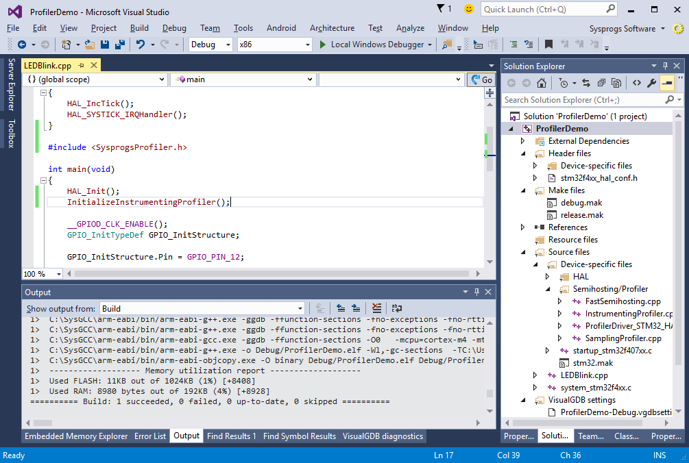
- Click “Analyze performance with VisualGDB” again and select “Instrument functions” in the setup window. VisualGDB will detect that your binary does not contain the relocation records required by the profiler and will suggest fixing this automatically. Select “Yes” to apply the fix and build your project again:
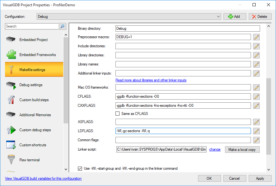
- You can double-check that the relocation generation is enabled via VisualGDB Project Properties. The “-Wl,-q” option should be present in the Linker Settings:
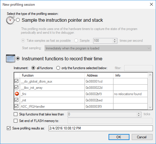
- Now you can finally start the instrumenting session. Proceed with the default option of instrumenting all functions:
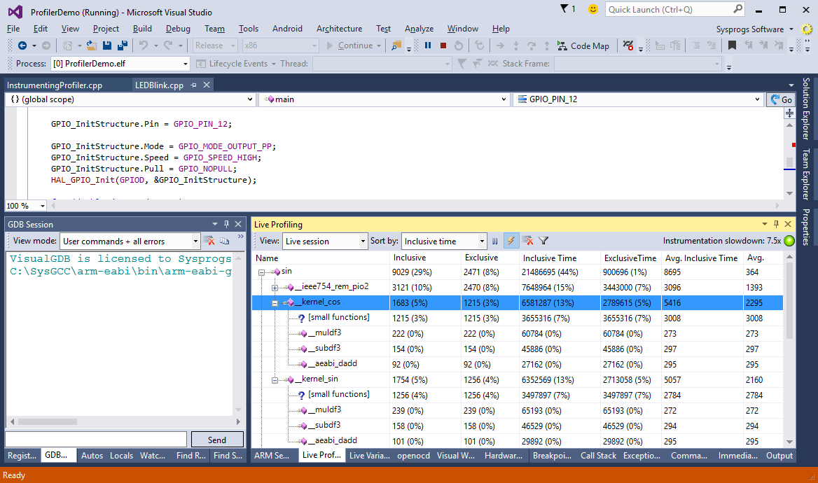
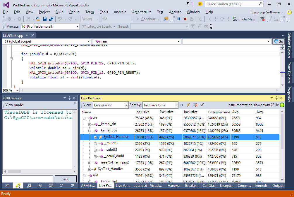
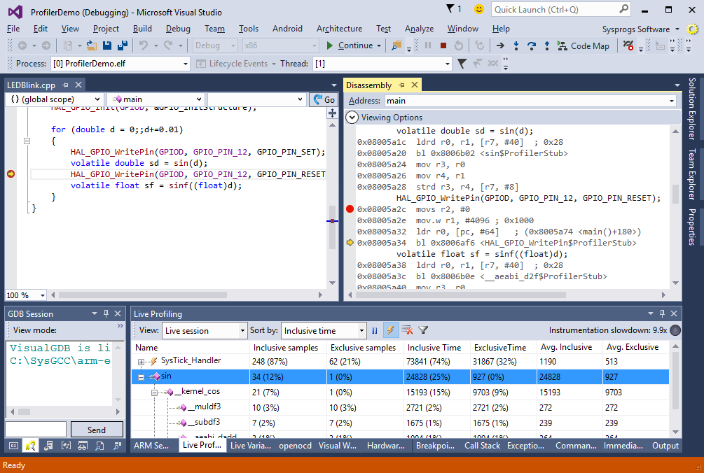
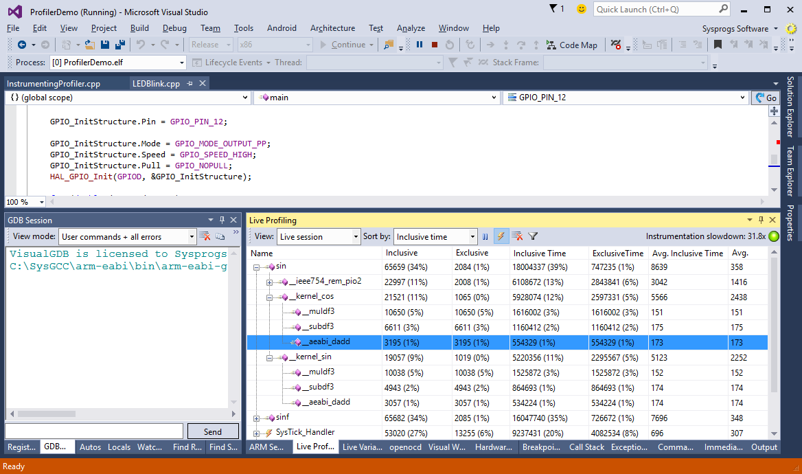
- VisualGDB will start a debugging session and display the real-time performance information in the Live Profiling window:
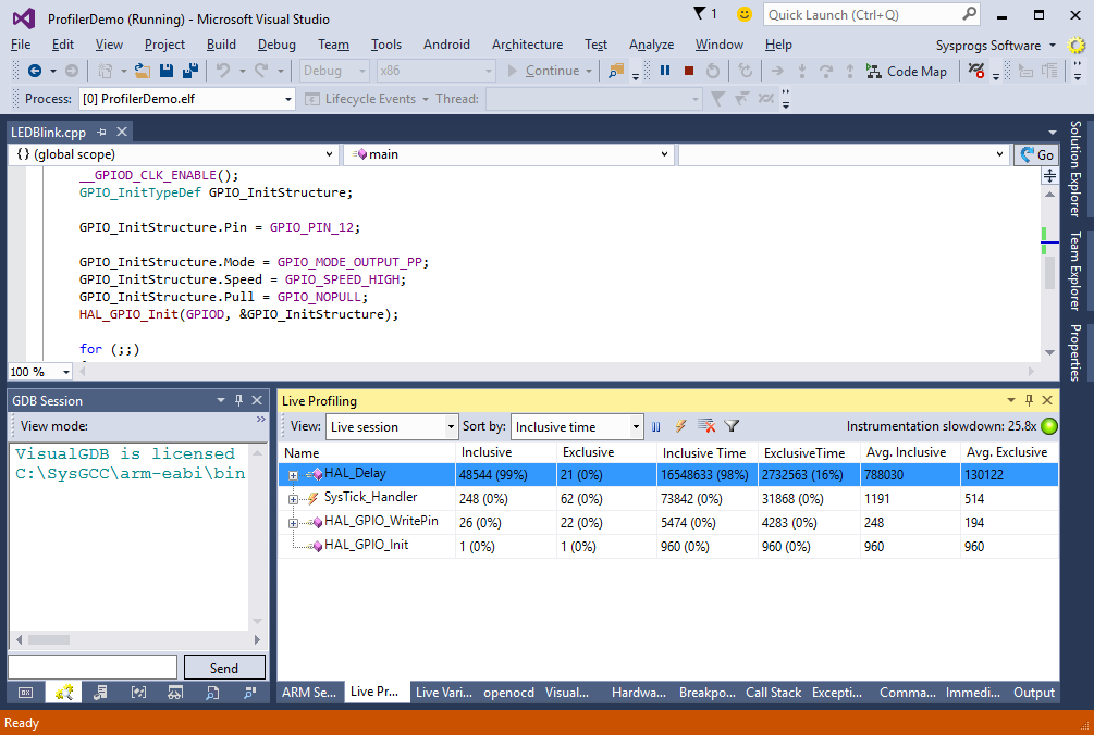 The “inclusive samples” column shows how many times a given function and any function called by it was invoked during profiling. The “exclusive samples” shows the exact amount of invocations for the function itself. The “Inclusive time” column shows the total time spent inside the function and any functions called by it. The “exclusive time” shows how much time was spent by the function itself. The time values are measured in ticks that normally correspond to the values of the debug cycle counter. We will show later how the ticks are counted.
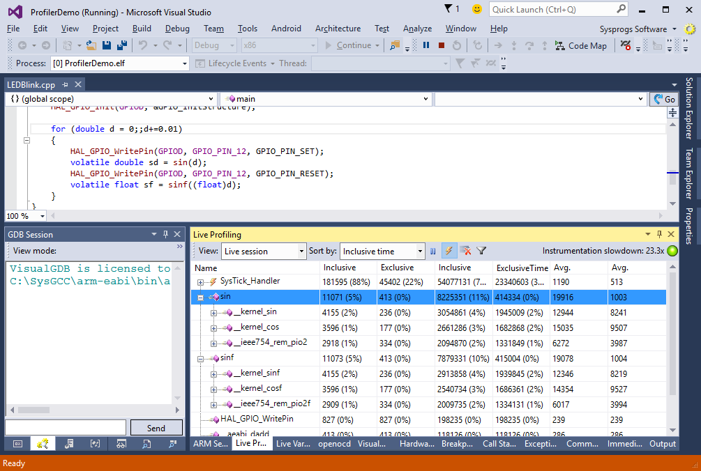
 - We will now use the instrumenting profiler to compare the performance of the sin() and sinf() functions. Both compute the sine of the argument, however one of them uses reduced-precision 32-bit numbers instead of 64-bit ones. Modify the loop inside main() as shown below:
for (double d = 0;;d+=0.01)
{
    volatile double sd = sin(d);
    volatile float sf = sinf((float)d);
}
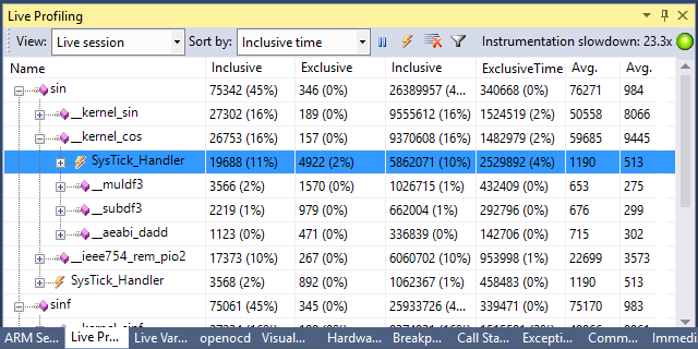
- Start the profiling session and observe the Live Profiling window:
- Note that some of the inclusive time of the sin() and sinf() functions comes from the SysTick interrupt handler that gets invoked while the function is running. VisualGDB automatically detects when an interrupt is invoked and allows filtering out the interrupt time. Click the button with the lightning icon. You will see that all the invocations of the interrupt handler has been combined into a separate entry and the times of normal functions don’t include interrupts anymore:
 Note that the interrupt handler takes a lot of time as we have not switched our device to the fast clock and the code execution is relatively slow compared to the rate of SysTick interrupts
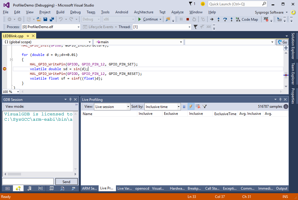
 - You can also use the instrumentation profiling to get precise measurements from single function invocations. Set a breakpoint just before a call to sin() and clear the Live Profiling window contents:
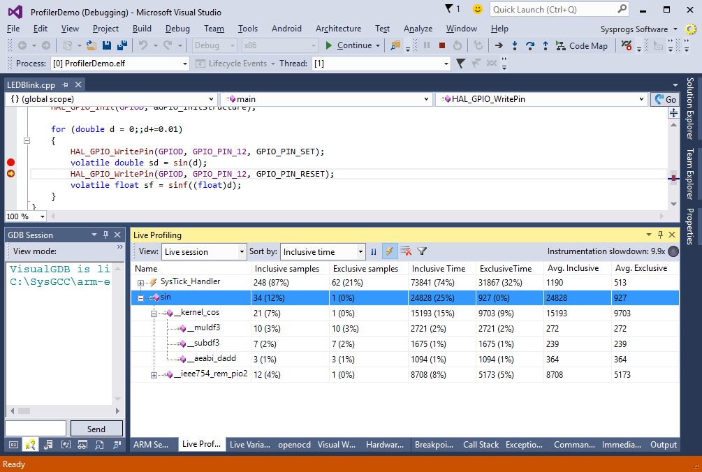
- Set a breakpoint on the next line and press F5 (single-stepping with F10 will result into several single-instruction steps and may result in extra interrupts being raised). The Live Profiling will display the exact information about all function calls that happened before the new breakpoint hit and the time of each call:
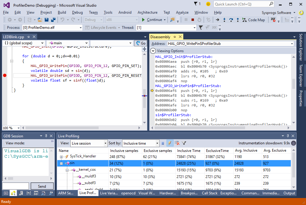
- Now we will show how the profiler tracks function calls. Switch to the disassembly view and try stepping into any function call:
- Observe that instead of calling the original functions like sin or HAL_GPIO_WritePin() the code calls generated functions like HAL_GPIO_WritePin$ProfilerStub. Each stub simply invokes the profiler hook that wraps the original function with the performance measurement code:
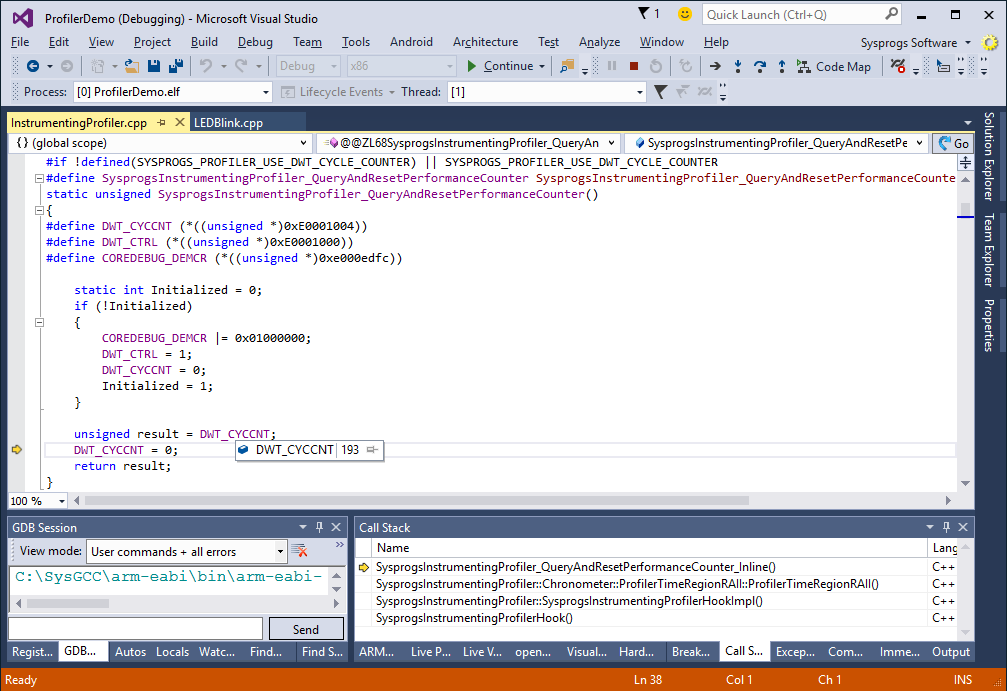
- The performance measurement code relies on the SysprogsInstrumentingProfiler_QueryAndResetPerformanceCounter() function to get the timings of the functions. You can replace the debug cycle counter with any other hardware counter, as long as it has enough width not to overflow while your code is running some long branch without any function calls and hence is not invoking the profiler:
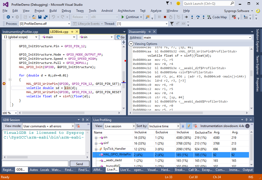
- If your code contains a lot of small functions, the overhead of measuring the performance of each one can be significant. The profiler actually estimates the slowdown caused by it by timing its own code and comparing it to the application code timings. The slowdown coefficient is shown at the right of the Live Profiling window. Note that release builds usually result in lower overhead due to better optimization:
- You can reduce the overhead even further by filtering out the function calls that took too little time. They will be still measured, but won’t be reported to VisualGDB and hence won’t use the JTAG bandwidth. First of all, determine the cutoff point by looking at the inclusive times of the functions you want to exclude:
- Then click the filter icon and set a threshold to a value above the typical inclusive time of those functions:
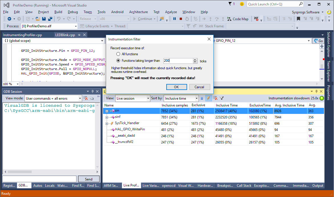
- Observe how the performance overhead significantly reduces and how the small functions are now grouped together: